Getting Started with pyDelta’s next branch

pyDelta’s next branch contains our work-in-progress implementation of experiments using Delta variants as a python library. We assume you have installed the library using pip.

First, let’s import the delta package:

import delta

Loading the corpus and preparing the feature matrix

The Corpus class represents the corpus as a bag-of-words feature matrix. In its simplest form, you can just call Corpus and pass it the directory your texts reside in:

raw_corpus = delta.Corpus('../../refcor/English')

This simple form assumes your texts in plain text files following the pattern Author_Title.txt. The reference corpora of English, French and German novels we use can be found on Github. If your corpus looks different, or if you need other ways of feature extraction than our simple tokenizer regular expression, have a look at the full documentation of our Corpus class for ways of parametrizing or further customizing feature extraction.

Corpus is simply a subclass of pandas’ DataFrame. The rows represent the documents, the columns the individual types. Let’s look at the Corpus’ top left corner:

print(raw_corpus.shape)
raw_corpus.iloc[0:5,0:10]

(75, 87829)

	the	and	to	of	a	I	in	was	that	he
ward_ashe	6904.0	4523.0	3498.0	4071.0	3185.0	1859.0	2278.0	1928.0	1528.0	1466.0
blackmore_springhaven	9965.0	6555.0	5865.0	6539.0	4637.0	2896.0	2449.0	2156.0	2572.0	2244.0
stevenson_island	4075.0	2680.0	1508.0	1671.0	1720.0	1965.0	932.0	1130.0	857.0	808.0
thackeray_esmond	9742.0	7992.0	4907.0	5541.0	4158.0	1898.0	2981.0	2755.0	2432.0	2385.0
ward_milly	2098.0	2189.0	1262.0	716.0	1058.0	596.0	565.0	563.0	364.0	298.0

The matrix contains the absolute frequencies of each word in each document, columns are sorted by the sum of all absolute frequencies.

Corpus has a few methods to manipulate the feature matrix, e.g., to perform culling: To remove all tokens that are not present in at least ⅓ of all documents, use

culled_corpus = raw_corpus.cull(1/3)
print(culled_corpus.shape)

(75, 10039)

Unless documented otherwise, these method return a new modified corpus instead of changing the current one.

For most experiments, you’ll want to work on the relative frequencies of the :math:`n most frequent words <delta.html#corpus.Corpus.topn>`__. There is a combined method for that:

c2500 = raw_corpus.get_mfw_table(2500)

Using delta functions to create a distance matrix

pydelta provides a number of delta functions by name that all produce a distance matrix. To run, e.g., Cosine Delta on our corpus from above:

distances = delta.functions.cosine_delta(c2500)
distances.iloc[:5,:5]

	ward_ashe	blackmore_springhaven	stevenson_island	thackeray_esmond	ward_milly
ward_ashe	0.000000	1.172292	1.102327	1.036012	1.014371
blackmore_springhaven	1.172292	0.000000	0.901935	0.949230	0.999159
stevenson_island	1.102327	0.901935	0.000000	1.059726	0.874804
thackeray_esmond	1.036012	0.949230	1.059726	0.000000	1.082447
ward_milly	1.014371	0.999159	0.874804	1.082447	0.000000

It is possible to run a few evaluations already on the distance matrix:

distances.evaluate()

F-Ratio         0.405758
Fisher's LD     1.328287
Simple Score    3.613850
dtype: float64

F-Ratio and Fisher’s Linear Discriminant are established measures (see Heeringa et al., 2008), to calculate the Simple Score we first standardize the distances and then calculate the difference between the mean distances between out-group and in-group texts (i.e., texts by different authors and texts by the same author).

You can also get the distances as a flat table. This will effectively return a flattened version of the lower right triangle of the distance matrix above, as scipy.spatial.distance.squareform(distances) would do, but with a proper index:

distances.delta_values()

ward_ashe          blackmore_springhaven    1.172292
                   stevenson_island         1.102327
                   thackeray_esmond         1.036012
                   ward_milly               1.014371
                   burnett_lord             0.953704
                                              ...
james_muse         lytton_novel             0.989467
                   doyle_lost               1.054597
james_ambassadors  lytton_novel             1.017272
                   doyle_lost               0.982058
lytton_novel       doyle_lost               1.064256
Name: cosine_delta, Length: 2775, dtype: float64

Clustering results

It is common to use clustering on the basis of the distance matrix in order to group similar texts. pydeltas Clustering class is a convenience wrapper around hierarchical clustering methods, of which Ward clustering is the default:

clustering = delta.Clustering(distances)

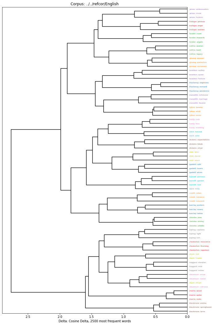
A hierarchical clustering is typically visualized using a Dendrogram. We’ve included an implementation that colors by author and provides labels using the DocumentDescriber that is assigned when creating the corpus:

import matplotlib.pyplot as plt
plt.figure(figsize=(10,15))
delta.Dendrogram(clustering).show()

/home/tv/git/pydelta/delta/graphics.py:88: MatplotlibDeprecationWarning: Passing the pad parameter of tight_layout() positionally is deprecated since Matplotlib 3.3; the parameter will become keyword-only two minor releases later.
  plt.tight_layout(2)

For any but a visual inspection, it is probably best to cut through the hierarchical clustering to provide flat clusters. This can be done with default settings from the hierarchical clustering:

clusters = clustering.fclustering()
print(clusters.describe())

25 clusters of 75 documents (ground truth: 25 groups):
{1: ['blackmore: springhaven', 'blackmore: erema', 'blackmore: lorna'],
 2: ['morris: water', 'morris: roots', 'morris: wood'],
 3: ['stevenson: island', 'stevenson: arrow', 'doyle: micah',
     'stevenson: catriona'],
 4: ['haggard: mist', 'haggard: sheallan', 'haggard: mines'],
 5: ['doyle: hound', 'doyle: lost'],
 6: ['chesterton: napoleon', 'chesterton: thursday', 'chesterton: innocence'],
 7: ['kipling: kim', 'kipling: light', 'kipling: captains'],
 8: ['cbronte: shirley', 'cbronte: villette', 'cbronte: jane'],
 9: ['barclay: ladies', 'barclay: rosary', 'barclay: postern'],
 10: ['corelli: innocent', 'corelli: romance', 'corelli: satan'],
 11: ['ward: milly', 'burnett: lord', 'burnett: garden', 'burnett: princess'],
 12: ['gaskell: lovers', 'gaskell: ruth', 'gaskell: wives'],
 13: ['eliot: adam', 'eliot: daniel', 'eliot: felix'],
 14: ['dickens: bleak', 'dickens: oliver', 'dickens: expectations'],
 15: ['ward: ashe', 'ward: harvest'],
 16: ['hardy: tess', 'hardy: jude', 'hardy: madding'],
 17: ['lytton: what', 'lytton: kenelm', 'lytton: novel'],
 18: ['meredith: marriage', 'meredith: feverel', 'meredith: richmond'],
 19: ['thackeray: esmond', 'thackeray: pendennis', 'thackeray: virginians'],
 20: ['braddon: fortune', 'braddon: quest', 'braddon: audley'],
 21: ['gissing: warburton', 'gissing: unclassed', 'gissing: women'],
 22: ['collins: basil', 'collins: woman', 'collins: legacy'],
 23: ['forster: angels', 'forster: howards', 'forster: room'],
 24: ['trollope: angel', 'trollope: warden', 'trollope: phineas'],
 25: ['james: hudson', 'james: muse', 'james: ambassadors']}

There are also some measures of cluster quality built into our class:

clusters.evaluate()

Cluster Errors         2.000000
Adjusted Rand Index    0.932358
Homogeneity            0.981365
Completeness           0.984136
V Measure              0.982749
Purity                 0.973333
Entropy                0.018635
dtype: float64